Scientific Computing
Contents
Scientific Computing
Scientific Python: Scipy Stack
Scipy = Scientific Python
scipynumpypandasData Analysis in Python
Scipy is an ecosystem, including a collection of open-source packages for scientific computing in Python.
A ‘family’ of packages that all work well together to do scientific computing.
Not made by the same people who manage the standard library.
Homogenous Data
for example: store data of the same type (i.e. all numerics)
recordings of values from experimental participants
heights or quantitative information from survey data
Lists are a start, and lists of lists are possible.
But, they can get nightmareish.
So we use arrays.
numpy
numpy - stands for numerical python
arrays - work with arrays (matrices)
Allow you to efficiently operate on arrays (linear algebra, matrix operations, etc.)
import numpy as np
# Create some arrays of data
arr0 = np.array([1, 2, 3])
arr1 = np.array([[1, 2], [3, 4]])
arr2 = np.array([[5, 6], [7, 8]])
arr1
array([[1, 2],
       [3, 4]])
# lists of lists don't store dimensionality well
[[1, 2], [3, 4]]
Indexing Arrays
# Check out an array of data
arr1
# Check the shape of the array
arr1.shape
# Index into a numpy array
arr1[0, 0]
Working with N-dimensional (multidimensional) arrays is easy within numpy.
Notes on Arrays
# arrays are most helpful when they
# have the same length in each list
np.array([[1, 2, 3, 4], [2, 3, 4]])
# arrays are meant to store homogeneous data
np.array([[1, 2, 'cogs18'], [2, 3, 4]])
Working with Arrays
(Things you can’t do with lists)
# Add arrays together
arr1 + arr2
# Matrix mutliplication
arr1 * arr2
A brief aside: zip()
zip() takes two iterables (things you can loop over) and loop over them together.
for a, b in zip([1,2], ['a','b']):
    print(a, b)
Clicker Question #1
Given the following code, what will it print out?
data = np.array([[1, 2, 3, 4],
                 [5, 6, 7, 8]])

output = []
for d1, d2 in zip(data[0, :], data[1, :]):
    output.append(d1 + d2)

print(output)
A) [1, 2, 3, 4]
B) [1, 2, 3, 4, 5, 6, 7, 8]
C) [6, 8, 10, 12]
D) [10, 26]
E) [36]
Note that if you find yourself looping over arrays…there is probably a better way.
data.sum()
data.sum(axis=0)
Heterogenous Data
have continuous (numeric) and categorical (discrete) data
different data types need to be stored
uses a DataFrame object (think: spreadsheet)
allows for column and row labels
pandas
import pandas as pd
# Create some example heterogenous data
d1 = {'Subj_ID': '001', 'score': 16, 'group' : 2, 'condition': 'cognition'}
d2 = {'Subj_ID': '002', 'score': 22, 'group' : 1, 'condition': 'perception'}
# Create a dataframe
df = pd.DataFrame([d1, d2], [0, 1])
# Check out the dataframe
df
| Subj_ID | condition | group | score | |
|---|---|---|---|---|
| 0 | 001 | cognition | 2 | 16 |
| 1 | 002 | perception | 1 | 22 |
# You can index in pandas
df['condition']
# You can index in pandas
df.loc[0,:]
Clicker Question #2
Comparing them to standard library Python types, which is the best mapping for these new data types?
A) DataFrames are like lists, arrays are like tuples
B) DataFrames and arrays are like lists
C) DataFrames are like tuples, arrays are like lists
D) DataFrames and arrays are like dictionaries
E) Dataframes are like dictionaries, arrays are like lists
Plotting
%matplotlib inline

import matplotlib.pyplot as plt
# Create some data
dat = np.array([1, 2, 4, 8, 16, 32])
# Plot the data
plt.plot(dat);
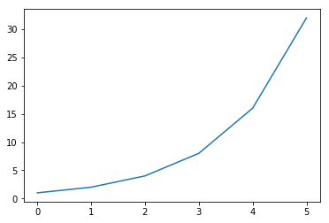
can change plot type
lots of customizations possible
Analysis
scipy- statistical analysissklearn- machine learning
import scipy as sp
from scipy import stats
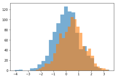
# Simulate some data
d1 = stats.norm.rvs(loc=0, size=1000)
d2 = stats.norm.rvs(loc=0.5, size=1000)
Analysis - Plotting the Data
# Plot the data
plt.hist(d1, 25, alpha=0.6);
plt.hist(d2, 25, alpha=0.6);
Analysis - Statistical Comparisons
# Statistically compare the two distributions
stats.ttest_ind(d1, d2)
Ttest_indResult(statistic=-9.33809588164776, pvalue=2.5256641524949454e-20)